Twine QAOA Service

In this tutorial we will demonstrate how to solve an optimization problem on quantum devices with the help of the ParityOS TwineQAOAService. We will cover the entire workflow; first the problem is reformulated by encoding it as the ground state of a Spin-Hamiltonian. By using the Parity Twine compilation the logical problem is mapped to a physical device where the respective quantum optimization algorithms can be run. From the output we then map back to the logical qubit configuration corresponding to the solution.

Problem Formulation

The problem we are going to tackle is an instance of MaxCut which has many important applications, e.g. in circuit design. We are given a graph \(G(V,E)\) with the nodes \(V\) and the edges \(E\) and the goal is to split the nodes into two sets such that as many edges as possible are cut (edges are cut if they connect nodes from different sets). Since it is NP-hard to even approximate the solution to this problem to arbitrary precision, it may be advantageous to solve it with the help of heuristic quantum algorithms. Our graph with 5 nodes and 6 edges connecting them looks as follows: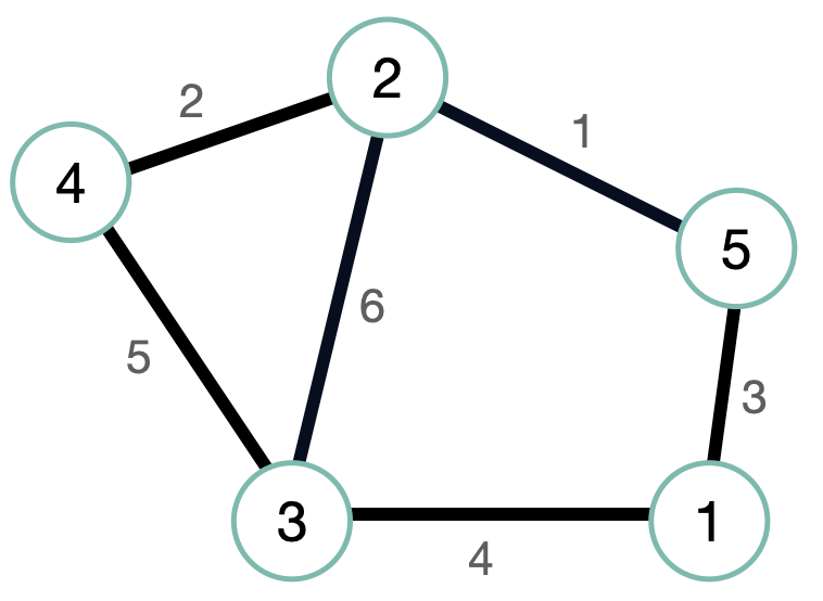

We now construct a Hamiltonian for solving the MaxCut problem on this graph so that the solution is encoded in the ground state. We assign a spin variable (qubit) \( s_i, i=1, ..., 5 \) to every node which takes the value +1 if the node belongs to the first set and -1 if it belongs to the second set. Since we want the solution to maximize the number of cut edges we use terms \( H_e \) that give a reward of -1 if the edge e is cut and a penalty +1 if not. This is achieved by simply adding a term \(H_e = s_i s_j\) for every edge \(e=(i, j)\) and thus \( H = \sum_{e \in E} H_e\) which we use to create an instance of the ProblemRepresentation class in ParityOS in the following format

from parityos.bits import get_q
from parityos.operators import Z
from parityos.optimization.problem_representation import ProblemRepresentation

logical_qubits = [get_q(i) for i in range(5)]
z = [Z(q) for q in logical_qubits]
# The interaction hamiltonian defining the optimization problems
hamiltonian = (
    1 / 2 * z[0] * z[4]
    + 1 / 2 * z[0] * z[2]
    + 1 / 2 * z[1] * z[4]
    + 1 / 2 * z[1] * z[2]
    + 1 / 2 * z[1] * z[3]
    + 1 / 2 * z[2] * z[3]
)

problem = ProblemRepresentation(hamiltonian)

Parity Twine Compilation

Next we use the Parity Twine compilation to map the logical problem onto a physical device. We first set up a device where our problem fits. In this case we choose a 2x3 rectangular device with nearest neighbor interactions

from parityos.devices.device_connectivity import get_rectangular_nearest_neighbor_connectivity
from parityos.devices.device_model import DeviceGate, DeviceModel, DeviceQubit
from parityos.operators import CNOT, RZ

dimensions = [2, 3]
nearest_neighbor_connectivity = get_rectangular_nearest_neighbor_connectivity(*dimensions)
native_operators = [DeviceGate(RZ(q)) for q in nearest_neighbor_connectivity.qubits] + [
    DeviceGate(CNOT(*connection.qubits))
    for connection in nearest_neighbor_connectivity.qubit_connections
    if len(connection) == 2
]
device_qubits = {DeviceQubit(qubit) for qubit in nearest_neighbor_connectivity.qubits}
device_model = DeviceModel(device_qubits, native_operators)

Then we set up a connection to the ParityOS cloud service using your username (password will be prompted or can be supplied via environment variables)

from parityos.services.authentication import InteractiveAuth
from parityos.services.client import HTTPClient

client = HTTPClient(InteractiveAuth("my_parityos_username"))  # handles authentication

The Twine compilation is invoked by instantiating the corresponding service, running it by passing the problem and device (and choosing 2 QAOA rounds) and extracting the parametrized QAOA circuit and the relabeling map that maps from the qubits on the physical device to the logical qubits of the problem

from parityos.services.service import TwineQAOAInput, TwineQAOAService

twine_qaoa_service = TwineQAOAService(client)
result = twine_qaoa_service.run(
    TwineQAOAInput(problem=problem, device=device_model), configuration={"num_rounds": 2}
)

param_circuit = result.parameterized_circuit
relabeling_map = result.relabeling_map

In order to run this circuit we first export it to the Qiskit format (also other backends are available)

from parityos_qiskit.exporter import export_parityos_to_qiskit

qiskit_circuit = export_parityos_to_qiskit(param_circuit).circuit
qiskit_circuit.measure_all()

Classical Optimization

Next we set up the classical optimization for which it is convenient to first define a helper function to compute the expectation value that is to be optimized from the counts, (i.e. the output of our simulated circuit). Note that counts is a dictionary containing the number of runs (values) in which the physical bitstring (keys) in binary variables was measured. We need to convert this physical bitstring to a quantum state in terms of the physical qubits for which we employ the function

def get_physical_state(bitstring):
    # Map the bits in the bitstring to 1 or 0 values for the physical qubits.
    qubit_to_value = {
        qubit: bool(int(bit)) for bit, qubit in zip(bitstring, param_circuit.ordered_qubits)
    }
    return PauliBasisState.from_qubit_to_value(qubit_to_value)

The helper function for the expectation value is defined as:

from parityos.evaluators import (
    PauliOperatorEvaluator,
    SingleProblemEvaluator,
    SoftConstraintEvaluator,
)
from parityos.states import PauliBasisState


def cost_expectation(counts, problem):
    expectation_sum = 0
    evaluator = SingleProblemEvaluator(
        operator_evaluator=PauliOperatorEvaluator(),
        constraint_evaluator=SoftConstraintEvaluator(1),
    )
    for bitstring, count in counts.items():
        physical_state = get_physical_state(bitstring)
        logical_state = PauliBasisState.from_qubit_to_value(
            {relabeling_map[qubit]: val for qubit, val in physical_state.qubit_to_value.items()}
        )

        cost = evaluator.evaluate_problem(logical_state, problem)
        expectation_sum += cost * count

    return expectation_sum / sum(counts.values())

Now we are able to execute the parametrized circuit with a simulator from Qiskit. For this we will construct a function that can be passed to a classical optimizer:

from qiskit.primitives import StatevectorSampler

def execute_circuit(parameters, parametrized_qiskit_circuit=qiskit_circuit):
    job = StatevectorSampler().run([(parametrized_qiskit_circuit, parameters)], shots=512)
    counts = job.result()[0].data.meas.get_counts()

    return cost_expectation(counts, problem)

Starting the optimization multiple times from random initial values for the QAOA parameters improves the performance, where we also set up the parameter bounds for the optimization of the angles.

import math

import numpy as np

parameter_bounds = {param: [-math.pi, math.pi] for param in qiskit_circuit.parameters}
n_starting_points = 5

initial_parameters, *initial_parameter_list = [
    [np.random.uniform(bound[0], bound[1]) for bound in parameter_bounds.values()]
    for _ in range(n_starting_points)
]

With these initial values the classical optimization is invoked with:

from scipy.optimize import minimize


def optimize_parameters(initial_parameters: list[float]) -> tuple[float, list[float]]:
    optimization_result = minimize(
        execute_circuit,
        x0=initial_parameters,
        bounds=[parameter_bounds[param] for param in qiskit_circuit.parameters],
        method="Nelder-Mead",
    )
    return optimization_result.fun, optimization_result.x


cost, optimal_parameters = optimize_parameters(initial_parameters)

for initial_parameters_candidate in initial_parameter_list:
    # call classical optimization method
    optimized_cost, optimized_parameters = optimize_parameters(initial_parameters_candidate)
    if optimized_cost < cost:
        # update parameters when associated cost is lower than previous best
        cost = optimized_cost
        optimal_parameters = optimized_parameters

Here we employ the Nelder-Mead optimizer from scipy, but other methods may also be used.

Solutions of the QAOA algorithm and decoding

So far we obtained the optimized parameters for our QAOA circuit. We now run it one more time with these parameters:

# assign optimized parameters to circuit
optimal_qaoa_circuit = qiskit_circuit.assign_parameters(optimal_parameters)

job = StatevectorSampler().run([optimal_qaoa_circuit])
counts = job.result()[0].data.meas.get_counts()

We select a number of physical bitstrings which were the most frequent outcomes of the circuit:

n_best_solutions = 5
best_physical_bitstrings = sorted(counts, key=counts.get, reverse=True)[:n_best_solutions]

best_physical_configurations = [
    get_physical_state(physical_bitstring) for physical_bitstring in best_physical_bitstrings
]

From these we get the candidates for the solution to the logical problem by decoding

logical_solution, *best_logical_states = [
    PauliBasisState.from_qubit_to_value(
        {relabeling_map[qubit]: val for qubit, val in state.qubit_to_value.items()}
    )
    for state in best_physical_configurations
]

Finally, the candidate solutions are evaluated on the logical Hamiltonian and we pick the best solution:

evaluator = SingleProblemEvaluator(
        operator_evaluator=PauliOperatorEvaluator(),
        constraint_evaluator=SoftConstraintEvaluator(1),
)

# initial cost
cost = evaluator.evaluate_problem(logical_solution, problem)

for logical_state in best_logical_states:
    # evaluate logical bitstring on logical Hamiltonian
    cost_of_bitstring = evaluator.evaluate_problem(logical_state, problem)
    # update logical solution if associated cost is lower than previous best
    if cost_of_bitstring < cost:  # pyright: ignore[reportOperatorIssue]
        logical_solution = logical_state
        cost = cost_of_bitstring

logical_solution.reorder(logical_qubits)
print("solution: ", logical_solution)

From the solution we can readily read off which nodes (represented by qubits) of the graph belong to which subset of the partition, e.g. 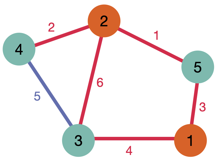where red edge labels indicate a cut edge and blue labels indicate an uncut edge. This problem instance is degenerate, meaning that there is more than one optimal solution. Therefore, and due to the probabilistic nature of the quantum algorithm running the code you might get a different result.